p(A|B)
=
p(B|A)
p(A)
p(B)

Let's take another look at Bayes' Theorem to recap its importance. Here it is again—as before, hover over any term in the equation for a summary of what that term means:
p(A|B)
=
p(B|A)
p(A)
p(B)
The posterior probability: The probability that A is true, based on some knowledge or observation B. It is called the "posterior" probability because posterior means later or after, and it is the probability of A after you have observed B.
The likelihood: The probability of your observation B, assuming that A is true.
The prior probability: The probability that A is true, without any other knowledge about the state of the world. It is called the "prior" probability because prior means before, and it is the probability of A before you have made your observation B.
There is no special name for this term, but you could refer to it as the normalizing constant. It is the probability of the observation B.
And here is Bayes' Theorem for our specific case:
p(black and blue | image)
=
p(image | black and blue)
p(black and blue)
p(image)
p(white and gold | image)
=
p(image | white and gold)
p(white and gold)
p(image)
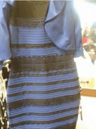
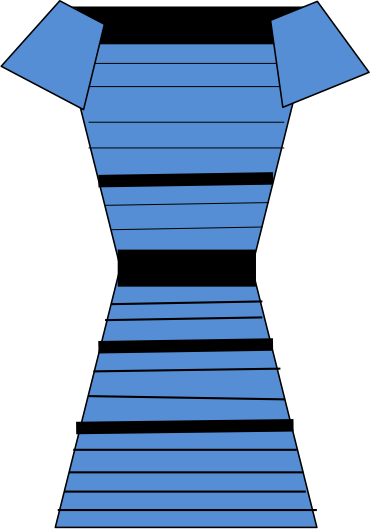
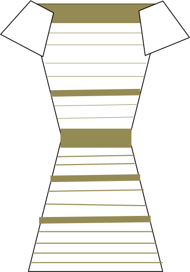
Bayes' Theorem is generally used to evaluate the probability of some hypothesis in light of some evidence. In this case, the hypothesis is that the dress is black and blue, and the evidence is the image, and the posterior probability, i.e. p(black and blue | image), expresses the probability of this hypothesis based on this evidence.
This posterior probability is in a form that we cannot directly evaluate, however, and this is where Bayes' Theorem comes to the rescue: it expresses this posterior probability in terms of other expressions that we can evaluate.
The two keys elements of our expanded expression are the likelihood, p(image | black and blue), and the prior probability, p(black and blue). The likelihood is the probability that we would observe our evidence (the image) assuming that our hypothesis is true, while the prior probability is the probability of our hypothesis being true without any evidence for or against it. Bayes' Theorem is useful in cases where we are able not able to directly model the posterior but are able to model the likelihood and the prior; and this turns out to cover many interesting areas of study in cognitive science as well as many other fields.
The final term of the equation is the normalizing constant, p(image). This term is necessary to ensure that, if we sum across the probabilities of all hypotheses, the total probability is 1.0.
To get more of a feel of how the prior probability, likelihood, and normalizing constant effect the posterior probability, play with the sliders below. (Technical note: We are acting as if, whenever you manually adjust the normalizing constant, the priors and likelihoods are scaled accordingly so as to preserve their ratios while generating the desired normalizing constant.)


Priors
Likelihoods
Normalizing constant
Did you notice how, when you crossed the posterior probability threshold between white/gold and black/blue, the woman's perception of the dress changed instantly? This is an example of categorical perception, a phenomenon where people automatically place continuous inputs into discrete bins.
Another thing you should have noticed is that changing the normalizing constant had no effect on the posterior probabilities. (If you didn't notice that, try it out with the sliders!) This makes sense if you look back at our versions of Bayes' Theorem expressed for the case of the dress: Both equations (the one for p(black and blue | image) and the one for p(white and gold | image)) have p(image) in their denominators. But for purposes of determining whether black/blue or white/gold has a higher posterior probability, we don't care about the absolute values of the posterior probabilities but rather about their relative values—i.e. which one is larger. This ranking is not affected by the value of the normalizing constant, because if we know that p(black and blue | image) > p(white and gold | image), it is also the case that c * p(black and blue | image) > p(white and gold | image) for any positive constant c. 1/p(image) is such a constant, so we can simply ignore it as long as all we care about is the relative ranking of the various posterior probabilities.
With this fact in mind, we can now rewrite Bayes' Theorem as follows:
p(A|B)
∝
p(B|A)
p(A)
The posterior probability: The probability that A is true, based on some knowledge or observation B. It is called the "posterior" probability because posterior means later or after, and it is the probability of A after you have observed B.
The likelihood: The probability of your observation B, assuming that A is true.
The prior probability: The probability that A is true, without any other knowledge about the state of the world. It is called the "prior" probability because prior means before, and it is the probability of A before you have made your observation B.
This symbol means "is proportional to," indicating that the left hand side is equal to the right hand side times some constant. In our case, the constant is 1/p(B)
You can paraphrase this version of the formula as "the posterior is proportional to the likelihood times the prior." If you remember from the first simulation, the normalizing constant was the most difficult thing to calculate because it involved summing over both possible scenarios (black/blue and white/gold). In more realistic problems, there are far more than just two possibilities to consider, so the calculation of the normalizing constant can go from being merely annoying to being completely untractable. For example, Gegenfurtner et al. 2015 found that there are not only two possible ways of interpreting the dress (black/blue vs. white/gold) but rather that, within these two broad categories, there are many distinct possibilities corresponding to different wavelengths of blue and gold, so to calculate the normalizing constant with this information we would have to sum across all these possible wavelengths. Therefore, this modified version of Bayes' Theorem is very useful as it eliminates the need to compute the potentially expensive normalizing constant. In the later simulations we will make use of this version of the formula.
Gegenfurtner, K. R., Bloj, M., & Toscani, M. (2015). The many colours of ‘the dress’. Current Biology, 25(13), R543-R544.